neural networks in cobol and other creative ways to k*ll yourself

Disclaimer: this is a tribute to the Cruelty Squad video game. Just to showcase how COBOL can still be used in bizarre ways to maximize shareholder value. ✨

---

Yesterday I opened my inbox expecting the usual sprint cosplay and jira fan fiction. Instead, I got a message from a guy that predates agile, devops, and most human rights:

Listen, employee. Your next assignment involves critical bio-surveillance operations: we have intercepted subversive penguins attempting to infiltrate corporate aquaculture infrastructure.

Your task is to classify these traitorous birds based on flipper length and other obscene morphological features.

BTW, you need to do it in COBOL (hope's is not a problem).

Do not disappoint me. The shareholders already do.

Naturally, I asked if I could at least sketch the thing in python first. I got this reply:

Fine. Babysit your little scripting language. But in the end, you return to the mainframe.

You always return to the mainframe.

Now classify those penguins before they unionize.

Alright. Let’s do this.

housekeeping

Before we dive in, I want to vehemently recommend the A Programmer’s Introduction to Mathematics book. It’s a great resource for anyone who wants to understand the math and speak symbols like the grown ups if you have a coding background like myself.

I also suggest taking a look at the 3Blue1Brown series on neural networks. They are very visual and build from the ground up.

We can download the Palmer penguin dataset from Kaggle.

neural what?

A neural network is just a function with knobs.

$$f_\theta(x) = y$$

You give it numbers. It outputs numbers.

The only thing you control is the parameters $\theta$. Training means adjusting those parameters so future outputs are less wrong than past ones.

There is no intelligence here. No understanding. The network does not know what it is doing. It only knows how to reduce a number called loss.

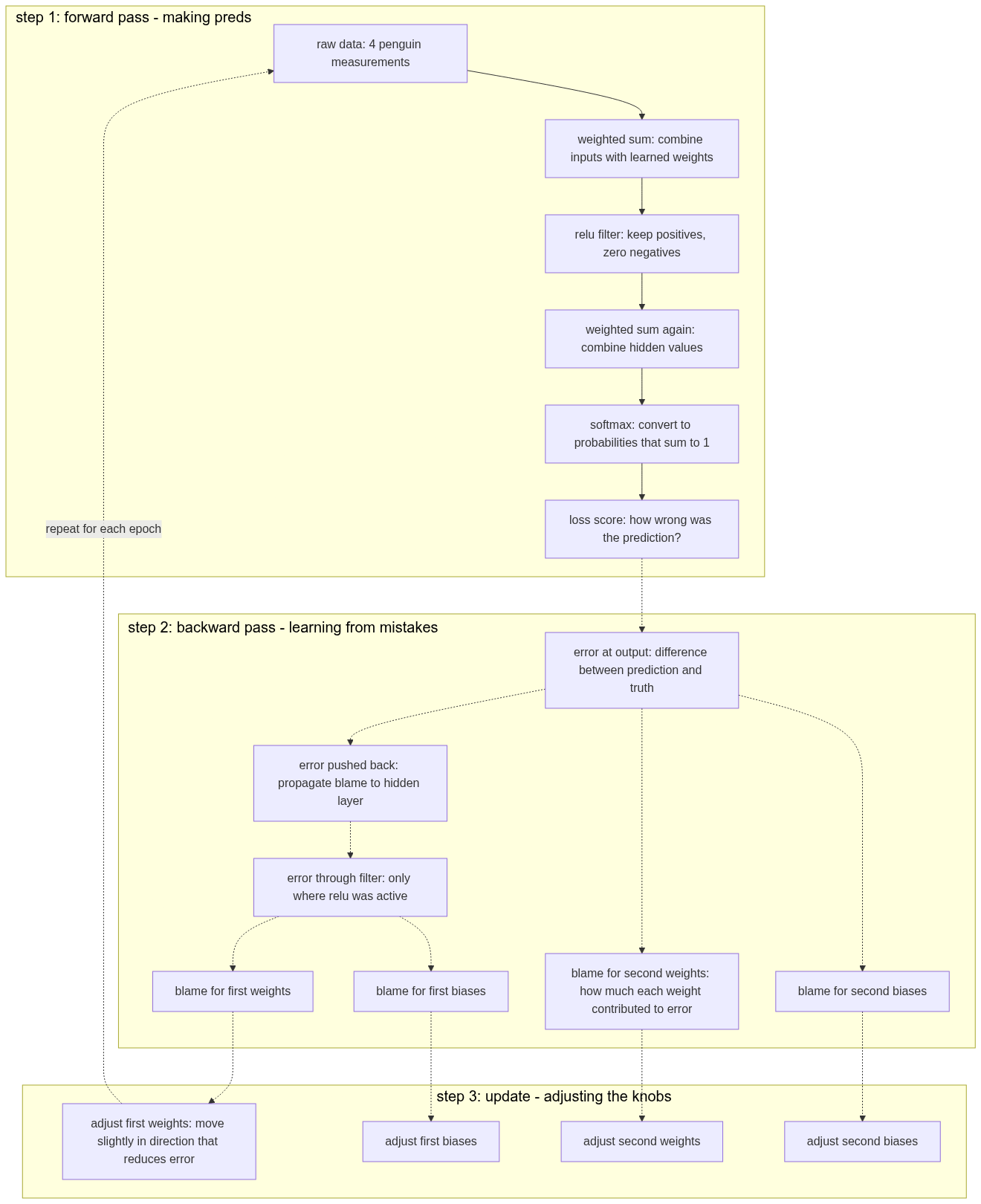
We’ll use the simplest non-trivial setup: a feedforward network with one hidden layer.

data as numbers, not vibes

The model never sees penguins. It sees vectors.

A vector is just a list of numbers arranged in a specific order. Think of it as coordinates in space, except instead of (x, y, z) you might have (bill_length, bill_depth, flipper_length, body_mass).

Your input is a fixed-length vector of measurements:

$$x = \begin{bmatrix} \text{bill length} \\ \text{bill depth} \\ \text{flipper length} \\ \text{body mass} \end{bmatrix} \in \mathbb{R}^4$$

This is 4-dimensional space. Each component is a real number.

Your target label is the species encoded as an integer (0 for Adelie, 1 for Chinstrap, 2 for Gentoo):

$$y \in \{0, 1, 2\}$$

So we're reducing living creatures to indices now? How delightfully reductive.

Yes. That is the point.

Before training, we normalize:

$$x' = \frac{x - \mu}{\sigma}$$

This subtracts the mean and divides by the standard deviation for each feature.

Why this matters: gradient descent assumes each dimension contributes on a similar scale. If one feature ranges in thousands and another in decimals, the optimizer zigzags and wastes steps.

the architecture

A neural network layer is two operations:

1. linear combination
2. nonlinear distortion

If you stack only linear layers, the whole network collapses into one linear transformation. Depth adds nothing. This is why nonlinearity is mandatory.

Hidden layer:

$$h = \text{ReLU}(xW_1 + b_1)$$

ReLU is the simplest useful nonlinearity:

$$\text{ReLU}(z) = \max(0, z)$$

It zeroes negative values and leaves positive ones unchanged. Without this, the network is just linear regression wearing a trench coat.

A trench coat? Is this neural network going to flash people at the park?

Different kind of exposure.

Output layer:

$$z_2 = hW_2 + b_2$$

These are raw scores called logits. They can be any real number.

Final step:

$$\hat{y} = \text{softmax}(z_2)$$

Softmax converts arbitrary scores into a probability distribution that sums to 1:

$$\text{softmax}(z_i) = \frac{e^{z_i}}{\sum_j e^{z_j}}$$

Shapes:

• $W_1 \in \mathbb{R}^{4 \times k}$ maps 4 inputs to k hidden units
• $b_1 \in \mathbb{R}^{k}$ offsets each hidden unit
• $W_2 \in \mathbb{R}^{k \times 3}$ maps hidden units to 3 classes
• $b_2 \in \mathbb{R}^{3}$ offsets class scores

turning wrong into a number

The model outputs probabilities. We need a single scalar that measures how bad the prediction is.

For classification, use cross entropy:

$$\mathcal{L}(y, \hat{y}) = -\sum_{i=1}^{3} y_i \log(\hat{y}_i)$$

Here $y$ must be converted from an integer index to a one-hot vector. This is a 3-dimensional vector where the true class gets a 1 and all others get 0. If the true class is 2 (Gentoo):

$$y = [0, 0, 1]$$

Why three dimensions? Because we have three species. The vector aligns with the three output probabilities $\hat{y} = [\hat{y}_1, \hat{y}_2, \hat{y}_3]$.

The loss reduces to:

$$-\log(\hat{y}_{\text{true}})$$

If the model assigns low probability to the correct class, the loss is large. If it is confidently wrong, the loss spikes. This is intentional. Wrong certainty should hurt more than uncertainty.

We're teaching the machine to feel pain through logarithms. This is either genius or the beginning of a very dark timeline.

Loss is the only feedback signal the network ever gets.

learning equals nudging numbers

Training means changing parameters to reduce loss.

The rule is gradient descent:

$$\theta \leftarrow \theta - \eta \nabla_\theta \mathcal{L}$$

The gradient points toward steeper loss. You step in the opposite direction.

$\eta$ is the learning rate. It controls step size.

Too small: training crawls. Too large: loss oscillates or explodes.

There is no universal value. You pick it empirically.

backpropagation, no mysticism

Backpropagation is the chain rule applied to the network graph.

The loss depends on the output. The output depends on the last layer. That depends on the hidden layer. That depends on the input layer.

Backprop computes gradients in reverse order. The notation looks scary but it is just derivatives:

$$\frac{\partial \mathcal{L}}{\partial W_2}, \frac{\partial \mathcal{L}}{\partial b_2}, \frac{\partial \mathcal{L}}{\partial W_1}, \frac{\partial \mathcal{L}}{\partial b_1}$$

Read $\frac{\partial \mathcal{L}}{\partial W_2}$ as “how much does loss change when I nudge $W_2$“. That curly $\partial$ symbol just means partial derivative, which is calculus for “change in this one thing while holding everything else constant”.

Nothing flows backward except these derivatives. They tell you which direction to adjust each parameter.

So backpropagation is just playing hot-and-cold with gradients until the loss stops screaming at you?

Essentially yes.

For softmax combined with cross entropy, the gradient simplifies beautifully:

$$\frac{\partial \mathcal{L}}{\partial z_2} = \hat{y} - y$$

full training loop

Training is boring and repetitive:

1. take a batch of inputs
2. compute predictions
3. compute loss
4. compute gradients
5. update parameters
6. repeat

If loss goes down, you are doing something right. If it does not, assume your setup is broken.

Six steps to artificial intelligence. What a time to be alive. I bet the researchers who spent decades on this love how you've reduced their life's work to "repeat until it works."

They should. It is accurate.

Let’s see the flow in context:

from english to python

Every operation becomes explicit code.

Linear transformation:

def linear(x, W, b):
    return x @ W + b

The @ symbol is matrix multiplication. It computes weighted sums of inputs. When you write x @ W, each row of x gets multiplied by each column of W and summed up. It is the same as writing nested loops, but readable.

ReLU and its derivative:

def relu(z):
    return np.maximum(0, z)

def relu_grad(z):
    return (z > 0).astype(float)

Softmax with numerical stability:

def softmax(z):
    exp = np.exp(z - np.max(z, axis=1, keepdims=True))
    return exp / np.sum(exp, axis=1, keepdims=True)

One-hot encoding for the target:

def one_hot(y, num_classes):
    out = np.zeros((len(y), num_classes))
    out[np.arange(len(y)), y] = 1
    return out

Cross entropy loss:

def cross_entropy(probs, y):
    return -np.mean(np.log(probs[np.arange(len(y)), y]))

Five functions. That's it? I've written longer code to format a date string.

Correct. The rest is just calling these repeatedly.

full working code

import numpy as np
import seaborn as sns
from sklearn.model_selection import train_test_split
from sklearn.preprocessing import StandardScaler

# data
df = sns.load_dataset("penguins").dropna()
X = df[["bill_length_mm", "bill_depth_mm", "flipper_length_mm", "body_mass_g"]].values
y = df["species"].astype("category").cat.codes.values

scaler = StandardScaler()
X = scaler.fit_transform(X)

X_train, X_test, y_train, y_test = train_test_split(
    X, y, test_size=0.2, random_state=42
)

# helpers
def relu(z):
    return np.maximum(0, z)

def relu_grad(z):
    return (z > 0).astype(float)

def softmax(z):
    exp = np.exp(z - np.max(z, axis=1, keepdims=True))
    return exp / np.sum(exp, axis=1, keepdims=True)

def one_hot(y, k):
    out = np.zeros((len(y), k))
    out[np.arange(len(y)), y] = 1
    return out

def cross_entropy(probs, y):
    return -np.mean(np.log(probs[np.arange(len(y)), y]))

# init
np.random.seed(0)
D = X.shape[1]
H = 16
C = len(np.unique(y))

W1 = np.random.randn(D, H) * 0.01
b1 = np.zeros(H)
W2 = np.random.randn(H, C) * 0.01
b2 = np.zeros(C)

lr = 0.1

# training
for epoch in range(150):
    # forward
    z1 = X_train @ W1 + b1
    h = relu(z1)
    z2 = h @ W2 + b2
    probs = softmax(z2)

    loss = cross_entropy(probs, y_train)

    # backward
    y_oh = one_hot(y_train, C)
    dz2 = probs - y_oh
    dW2 = h.T @ dz2 / len(X_train)
    db2 = dz2.mean(axis=0)

    dh = dz2 @ W2.T
    dz1 = dh * relu_grad(z1)
    dW1 = X_train.T @ dz1 / len(X_train)
    db1 = dz1.mean(axis=0)

    W1 -= lr * dW1
    b1 -= lr * db1
    W2 -= lr * dW2
    b2 -= lr * db2

    if epoch % 50 == 0:
        print(f"epoch {epoch}, loss {loss:.4f}")

# evaluation
z1 = X_test @ W1 + b1
h = relu(z1)
z2 = h @ W2 + b2
preds = np.argmax(softmax(z2), axis=1)

accuracy = (preds == y_test).mean()
print("test accuracy:", accuracy)

This outputs:

$ python pengu_nn.py 
epoch 0, loss 1.0987
epoch 50, loss 0.9576
epoch 100, loss 0.4045
test accuracy: 0.9701492537313433

Naturally, the Handler hates this.

Enough with your cheerful toy language. The mainframe thirsts.

Great.

the cobol nightmare

You want neural networks in COBOL? Enjoy the pain.

Well, I guess I have to dust off my ancient COBOL books¹:

COBOL was built for accountants, not gradient descent. You get fixed-width fields, no arrays the way you want them, no dynamic memory, and arithmetic that feels like chiseling numbers into wet clay.

Finally. A language that understands suffering. Python users have it too easy with their "readable syntax" and "helpful error messages."

I will show only the parts that correspond to neural network operations. For the full implementation including data loading, CSV parsing, train-test split, and all the WORKING-STORAGE boilerplate, see the complete source code.

data loading and preprocessing

COBOL loads CSV files line by line, validates against missing values, and encodes species as integers:

*    ENCODE TARGET SPECIES AS INTEGER LABELS (0-2).
EVALUATE WS-SPECIES-STR
    WHEN "Adelie"    MOVE 0 TO D-Y(WS-VALID-ROWS)
    WHEN "Chinstrap" MOVE 1 TO D-Y(WS-VALID-ROWS)
    WHEN "Gentoo"    MOVE 2 TO D-Y(WS-VALID-ROWS)
END-EVALUATE

Normalization is done with the same z-score formula, but spelled out explicitly:

*    STEP 5: APPLY Z-SCORE TRANSFORMATION TO ALL SAMPLES.
PERFORM VARYING IDX-ROW FROM 1 BY 1 
        UNTIL IDX-ROW > WS-VALID-ROWS
    COMPUTE D-X1(IDX-ROW) = (D-X1(IDX-ROW) - 
             WS-MEAN-X1) / WS-STD-X1
    COMPUTE D-X2(IDX-ROW) = (D-X2(IDX-ROW) - 
             WS-MEAN-X2) / WS-STD-X2
    COMPUTE D-X3(IDX-ROW) = (D-X3(IDX-ROW) - 
             WS-MEAN-X3) / WS-STD-X3
    COMPUTE D-X4(IDX-ROW) = (D-X4(IDX-ROW) - 
             WS-MEAN-X4) / WS-STD-X4
END-PERFORM

weight initialization

Python uses np.random.randn(). COBOL implements Gaussian sampling with the Box-Muller transform:

*    GAUSSIAN WEIGHT INITIALIZATION USING BOX-MULLER TRANSFORM.
*    G(X, Y) = SQRT(-2LN(U1)) * COS(2PI * U2).
PERFORM VARYING IDX-I FROM 1 BY 1 UNTIL IDX-I > 4
    PERFORM VARYING IDX-J FROM 1 BY 1 UNTIL IDX-J > 16
        COMPUTE WS-RAND-U1 = FUNCTION RANDOM
        COMPUTE WS-RAND-U2 = FUNCTION RANDOM
        COMPUTE WS-GAUSSIAN = 
            FUNCTION SQRT(-2 * FUNCTION LOG(WS-RAND-U1)) *
            FUNCTION COS(2 * WS-PI * WS-RAND-U2)
*       SCALE WEIGHTS DOWN (0.01) TO PREVENT GRADIENT EXPLOSION.
        COMPUTE W1-VAL(IDX-I, IDX-J) = WS-GAUSSIAN * 0.01
    END-PERFORM
END-PERFORM

Box-Muller transform. In COBOL. You're not just implementing a neural network, you're performing an exorcism.

forward pass: hidden layer

Python: z1 = X @ W1 + b1

COBOL: explicit nested loops for matrix multiplication.

*    HIDDEN LAYER COMPUTATION: Z1 = X * W1 + B1.
PERFORM VARYING IDX-J FROM 1 BY 1 UNTIL IDX-J > 16
    MOVE B1-VAL(IDX-J) TO Z1-VAL(IDX-I, IDX-J)
    COMPUTE Z1-VAL(IDX-I, IDX-J) = 
            Z1-VAL(IDX-I, IDX-J) +
            (D-X1(IDX-I) * W1-VAL(1, IDX-J))
    COMPUTE Z1-VAL(IDX-I, IDX-J) = 
            Z1-VAL(IDX-I, IDX-J) +
            (D-X2(IDX-I) * W1-VAL(2, IDX-J))
    COMPUTE Z1-VAL(IDX-I, IDX-J) = 
            Z1-VAL(IDX-I, IDX-J) +
            (D-X3(IDX-I) * W1-VAL(3, IDX-J))
    COMPUTE Z1-VAL(IDX-I, IDX-J) = 
            Z1-VAL(IDX-I, IDX-J) +
            (D-X4(IDX-I) * W1-VAL(4, IDX-J))

This is matrix multiplication, expressed as stubbornness.

forward pass: ReLU

Python: h = np.maximum(0, z1)

COBOL: an IF statement in a loop.

*    NON-LINEAR ACTIVATION: RELU(Z) = MAX(0, Z).
IF Z1-VAL(IDX-I, IDX-J) > 0
    MOVE Z1-VAL(IDX-I, IDX-J) TO H-VAL(IDX-I, IDX-J)
ELSE
    MOVE 0 TO H-VAL(IDX-I, IDX-J)
END-IF

forward pass: output layer

Python: z2 = h @ W2 + b2

COBOL: same pattern, different dimensions.

*    OUTPUT LAYER COMPUTATION: Z2 = H * W2 + B2.
PERFORM VARYING IDX-J FROM 1 BY 1 UNTIL IDX-J > 3
    MOVE B2-VAL(IDX-J) TO Z2-VAL(IDX-I, IDX-J)
    PERFORM VARYING IDX-K FROM 1 BY 1 UNTIL IDX-K > 16
        COMPUTE Z2-VAL(IDX-I, IDX-J) = 
                Z2-VAL(IDX-I, IDX-J) + 
                (H-VAL(IDX-I, IDX-K) * 
                 W2-VAL(IDX-K, IDX-J))
    END-PERFORM
END-PERFORM

forward pass: softmax

Python: vectorized exponentials and division.

COBOL: two-pass algorithm with explicit accumulation.

*    PROBABILITY ESTIMATION: SOFTMAX(Z2).
*    P_i = EXP(Z_i) / SUM(EXP(Z_j)).
COMPUTE P-VAL(IDX-I, 1) = FUNCTION EXP(Z2-VAL(IDX-I, 1))
COMPUTE P-VAL(IDX-I, 2) = FUNCTION EXP(Z2-VAL(IDX-I, 2))
COMPUTE P-VAL(IDX-I, 3) = FUNCTION EXP(Z2-VAL(IDX-I, 3))
MOVE 0 TO WS-TEMP-MATH
ADD P-VAL(IDX-I, 1) P-VAL(IDX-I, 2) P-VAL(IDX-I, 3) 
  TO WS-TEMP-MATH
COMPUTE P-VAL(IDX-I, 1) = P-VAL(IDX-I, 1) / WS-TEMP-MATH
COMPUTE P-VAL(IDX-I, 2) = P-VAL(IDX-I, 2) / WS-TEMP-MATH
COMPUTE P-VAL(IDX-I, 3) = P-VAL(IDX-I, 3) / WS-TEMP-MATH

Look at that. Three separate COMPUTE statements to normalize three probabilities. Inefficient? Yes. Beautiful? Also yes.

loss calculation

Python: loss = -np.mean(np.log(probs[range(n), y]))

COBOL: loop over samples, accumulate negative log probabilities.

*    CROSS-ENTROPY LOSS: L = -SUM(Y_TRUE * LOG(P_PRED)).
MOVE 0 TO WS-LOSS
PERFORM VARYING IDX-S FROM 1 BY 1 
        UNTIL IDX-S > WS-TRAIN-ROWS
    COMPUTE IDX-I = WS-IDX(IDX-S)
    COMPUTE IDX-J = D-Y(IDX-I) + 1
    COMPUTE WS-LOSS = WS-LOSS - 
                      FUNCTION LOG(P-VAL(IDX-I, IDX-J))
END-PERFORM
COMPUTE WS-LOSS = WS-LOSS / WS-TRAIN-ROWS

backpropagation: output gradient

Python: dz2 = probs - y_onehot

COBOL: copy probabilities, then subtract 1 from the true class.

*    DERIVATIVE OF SOFTMAX CW CROSS-ENTROPY: DZ2 = P - Y_TRUE.
PERFORM VARYING IDX-J FROM 1 BY 1 UNTIL IDX-J > 3
    MOVE P-VAL(IDX-I, IDX-J) TO BP-DZ2(IDX-J)
END-PERFORM
COMPUTE IDX-K = D-Y(IDX-I) + 1
SUBTRACT 1 FROM BP-DZ2(IDX-K)

backpropagation: W2 and b2 gradients

Python: dW2 = h.T @ dz2 / n and db2 = dz2.mean(axis=0)

COBOL: accumulate gradients across all samples, then average during update.

*    ACCUMULATE DW2 = H^T * DZ2 | DB2 = DZ2.
PERFORM VARYING IDX-J FROM 1 BY 1 UNTIL IDX-J > 3
    COMPUTE DB2-VAL(IDX-J) = DB2-VAL(IDX-J) + 
                             BP-DZ2(IDX-J)
    PERFORM VARYING IDX-K FROM 1 BY 1 UNTIL IDX-K > 16
        COMPUTE DW2-VAL(IDX-K, IDX-J) = 
                DW2-VAL(IDX-K, IDX-J) + 
                (H-VAL(IDX-I, IDX-K) * BP-DZ2(IDX-J))
    END-PERFORM
END-PERFORM

backpropagation: hidden layer gradient

Python: dh = dz2 @ W2.T

COBOL: explicit matrix-vector product.

*    BACKPROP TO HIDDEN LAYER: DH = DZ2 * W2^T.
PERFORM VARYING IDX-J FROM 1 BY 1 UNTIL IDX-J > 16
    MOVE 0 TO BP-DH(IDX-J)
    PERFORM VARYING IDX-K FROM 1 BY 1 UNTIL IDX-K > 3
        COMPUTE BP-DH(IDX-J) = BP-DH(IDX-J) + 
                (BP-DZ2(IDX-K) * W2-VAL(IDX-J, IDX-K))
    END-PERFORM

backpropagation: ReLU gradient

Python: dz1 = dh * (z1 > 0)

COBOL: IF statement as a gate.

*    DERIVATIVE OF RELU: DZ1 = DH IF Z1 > 0 ELSE 0.
IF Z1-VAL(IDX-I, IDX-J) > 0
    MOVE BP-DH(IDX-J) TO BP-DZ1(IDX-J)
ELSE
    MOVE 0 TO BP-DZ1(IDX-J)
END-IF

backpropagation: W1 and b1 gradients

Python: dW1 = X.T @ dz1 / n

COBOL: accumulate outer products.

*    ACCUMULATE DW1 = X^T * DZ1 | DB1 = DZ1.
COMPUTE DB1-VAL(IDX-J) = DB1-VAL(IDX-J) + 
                         BP-DZ1(IDX-J)
IF BP-DZ1(IDX-J) NOT = 0
    COMPUTE DW1-VAL(1, IDX-J) = 
      DW1-VAL(1, IDX-J) + 
      (D-X1(IDX-I) * BP-DZ1(IDX-J))
    COMPUTE DW1-VAL(2, IDX-J) = 
      DW1-VAL(2, IDX-J) + 
      (D-X2(IDX-I) * BP-DZ1(IDX-J))
    COMPUTE DW1-VAL(3, IDX-J) = 
      DW1-VAL(3, IDX-J) + 
      (D-X3(IDX-I) * BP-DZ1(IDX-J))
    COMPUTE DW1-VAL(4, IDX-J) = 
      DW1-VAL(4, IDX-J) + 
      (D-X4(IDX-I) * BP-DZ1(IDX-J))
END-IF

Four separate accumulation statements. One for each input feature. Because COBOL doesn't believe in shortcuts or happiness, kek.

parameter update

Python: W -= lr * dW

COBOL: compute scaled learning rate once, then apply to all parameters.

*    PERFORM PARAMETER UPDATES: PARAM = PARAM - LR * GRADIENT.
COMPUTE WS-TEMP-MATH = WS-LR / WS-TRAIN-ROWS
PERFORM VARYING IDX-I FROM 1 BY 1 UNTIL IDX-I > 16
    PERFORM VARYING IDX-J FROM 1 BY 1 UNTIL IDX-J > 3
        COMPUTE W2-VAL(IDX-I, IDX-J) = 
                W2-VAL(IDX-I, IDX-J) - 
                (WS-TEMP-MATH * DW2-VAL(IDX-I, IDX-J))
    END-PERFORM
    COMPUTE B1-VAL(IDX-I) = B1-VAL(IDX-I) - 
                            (WS-TEMP-MATH * DB1-VAL(IDX-I))
END-PERFORM

evaluation

Inference is the same forward pass without gradients. Prediction is argmax:

*    PREDICATE SELECTION: ARGMAX PROBABILITY.
EVALUATE TRUE
    WHEN P-VAL(IDX-I, 1) >= P-VAL(IDX-I, 2) AND 
         P-VAL(IDX-I, 1) >= P-VAL(IDX-I, 3)
        MOVE 0 TO WS-PRED-CLASS
    WHEN P-VAL(IDX-I, 2) >= P-VAL(IDX-I, 1) AND 
         P-VAL(IDX-I, 2) >= P-VAL(IDX-I, 3)
        MOVE 1 TO WS-PRED-CLASS
    WHEN OTHER
        MOVE 2 TO WS-PRED-CLASS
END-EVALUATE

grand finale

To compile these 578 lines of pure madness, just keep calm and use gnucobol:

$ cobc -x -o pengu_nn pengu_nn.cob && ./pengu_nn
LOADED 0333 VALID ROWS.
DATA HOUSEKEEPING COMPLETED.
EPOCH 0000 LOSS: +000000001.098705953
EPOCH 0050 LOSS: +000000000.948385870
EPOCH 0100 LOSS: +000000000.404952448
EPOCH 0150 LOSS: +000000000.254336047
EPOCH 0200 LOSS: +000000000.157729394
EPOCH 0250 LOSS: +000000000.097222933
EPOCH 0300 LOSS: +000000000.067910843
EPOCH 0350 LOSS: +000000000.052804836
EPOCH 0400 LOSS: +000000000.043876194
EPOCH 0450 LOSS: +000000000.037968264
EPOCH 0500 LOSS: +000000000.033755593
TEST ACCURACY: +000000001.000000000
TRAIN ACCURACY: +000000000.988721804

Does it work? Yes. Painfully. Slowly. Correctly.

I know what you are thinking: why on earth I put 500 epochs for such a small dataset? Coz’ we can. 😎

Perfect accuracy on the test set. Either you've achieved machine learning nirvana or you've overfitted so hard the penguins are filing a restraining order.

Anyway. Fair enough. The penguin insurgency will be contained... for now.

The penguins get classified. The loss goes down. The mainframe hums in approval. Somewhere, a finance department nods without understanding why.

---

You can find the full working code, including all the ugly declarations I spared you from, in this github repo.

1. yep, I know we don’t need IMS here. I just wanted to flex with that since I don’t get many chances, lol. ↩